Revisiting the Sternocleidomastoids: Accessory Muscles of Respiration

We know that sternocleidomastoids (strap muscles of the neck), scalene muscles and alae nasi are considered accessory muscles of breathing, although some controversy exists. If you saw an asthmatic individual in his desperate attempts at breathing or an agitated person or a person exercising vigorously, you could watch these muscles in action. However, that wasn't exactly what I had in mind while I was doing this experiment. I was really thrilled to chance upon it. Kind of a serendipitous discovery in its own right. You too can figure this out easily. The placement of the surface leads were as shown on the right. Red dots were for the reference and recording electrodes whereas the blue dot represents the ground (as usual). 

The neck muscles of each side were tested one at a time. For example, This wav file (open it Audacity or BYB neuron recorder) was obtained from EMG recording from the right sternocleidomastoid; the leads were placed on the right side and the ground lead on the manubrium. The head was at mid-line (neutral position) to start with. Next, it was turned to the right, then midline again, then to the left (without any external resistance applied), then against resistance applied by the left hand. The muscle of the right side moves the head to the left. Finally, the head was again restored in its neutral position. An improvised notation could be N to R to N to L to L+ to N (Legend: N=neutral, R = right, L=left, L+ = left against resistance). 

Similarly, the left side was tested in a likewise manner (N to L to N to R to R+ to N). And this is the waveform obtained. The surprise awaited me, I was in for an ambush!

While the leads were still on the strap muscles of the left side of my neck, I observed the EMG waveform in real-time. I noticed that as I was taking a deep breath, the EMG activity increased significantly. I didn't have to turn to my head to the right anymore! I then maintained this position by holding my breath. The activity continued. Here's the recorded .wav file. The associated camera recording will speak for it (see below: Youtube). Yes, it proved that it was indeed an accessory muscle called in to address forceful inhalation. I then did a forceful exhalation, but no increase in EMG activity was observed, buttressing my observation. 



As you may have noticed that I have used the terms inhalation and exhalation, in lieu of, inspiration and expiration. Well, inspiration, it definitely is! Expiration? No way!
Further analysis still awaits.
Spikerbox recordings may also possibly illustrate simultaneous EMG activities in protagonist and antagonist muscles. More of these later.

To be continued............

This work by Amiya Sarkar is licensed under a Creative Commons Attribution 4.0 International License.

Last modified: never 
Reference: hyper-links, unless specifically mentioned

Surface EMG from Thumb: Strongly 'Opposed' ?

Lead placement for the experiment, as shown on the right.
As I have already mentioned, the ground electrode sits atop
the manubrium sterni, on the upper chest (breastbone).

The camera recording is shown below. You can see the Piezoelectric crystal's spark and also hear its sound on snapping. However, I haven't yet had time to analyze if the spark did contribute some 'useful' static on the trace (open & watch this .wav file in BYB software).






Method: Pressing on a piezo crytal (from a cigarette lighter) by 'opposing' the thumb against the base of the little finger (as shown by the figure). Electrode placement shown in red & green markings [the ground electrode sits atop manubrium sterni]. Muscle (mainly) contracting is "opponens pollicis", a small, triangular muscle in the hand, which functions to oppose the thumb. [Strictly speaking, opposition of the thumb refers to the tip of the thumb touching the tips of other fingers. But that way, generating enough force without creating an unnecessary torque that topples the piezo is quite a challenge! After all, I had no assistant, and had to hold the camera too with the other hand]

Concept: A fixed and constant amount of force is necessary each time before the spring yields and the piezo fires. This end point is supposed to be caught in the trace 1) as a sharp spike after the surface EMG pattern or, 2) can be 'used' as a 'static'.

EMG amplitude and rate of spikes will need to be analyzed in short, discrete time intervals by simple counting.


This work by Amiya Sarkar is licensed under a Creative Commons Attribution 4.0 International License.
Last modified: never
Reference: hyper-links, unless specifically mentioned

Interpreting Rate Coding Data: Counting Spikes in a Tracing & Consequent Plotting of Firing Rate Versus Time

We acquire data by using the following device configuration (the green laptop cable will go to the laptop mic input, running on battery power) as shown below. Please see this link to learn about the anatomy of a coaxial cable, so that you can make a ground connection off a coaxial cable.

You can also take the ground off the reference point used for the Faraday cage clip, if you'd like. Incoming analog signals from the spikerbox will go into the internal ADC (Analog to Digital Converter) of the Conexant HD audio port of the laptop, whence the signal will be digitally processed. After a signal has been stored either in Audacity or in the BYB neuron recorder, we can open the'.aup' or the '.wav' file respectively later.

Here, I am attaching a typical wav file captured by striking the quadriceps tendon with a percussion hammer (knee jerk). This is a deep (tendon) reflex. I'll post more on this later. You need to open it using either of the two softwares listed. I am posting a screenshot on the right.
You can see three large spikes in the tracing. These spikes are actually not single/solitary, as they might innocuously suggest, but they are a conglomeration of many individual ones.

The below tutorial explains how to interpret these raw data.



By the way, there's no simple way to count spikes! First, we need to define spikes. We can fix an arbitrary threshold, beyond which we will label them as one. Here are some very rudimentary thoughts on counting:

• Coupling/buffering the output from the laptop audio-out port via ICs like ULN 2004 Darlington transistor arrays to drive filament lamps [these filament lamps are a modest way to an integrator as the heat takes time to dissipate off]. The more the spike rates, greater will be the brightness. Then pick-up this optical signal by an LDR (Light Dependent Resistor) and then noting the resistance change [precalibration is necessary]. We can use capacitors too (using their exponential charging/discharging equations) or a linear optocoupler like MOC5010.
• Software: writing some code snippets to Matlab/Python programs 
• Using a Foster-Seeley phase discriminator: However, a new algorithm should be developed.
• Converting the electrical signals to mechanical tracings on a rotating Kymograph [speed adjusted] may make it easier to read and count
• Allowing only signals above a certain 'predefined' threshold voltage to pass through. We may use diodes for this cut-off estimation. Next, employ a CD 4520, a dual 4 BIT binary up counter that advances from LOW to High transition on clock input '0' (CK0) when CK1 is high, after the signal has been "gate"d . We can use an appropriate crystal to this counting purpose. Many optically based circuits are available on the net.
• We can think of using a frequency to voltage converter IC like LM 2907
• But presently, i'll be counting them manually. My time limitations and fading electronic experiences precludes any pursuits of above kind.

After we have successfully counted the 'rates' of 'action potential's, we can plot their number/spikes vs time plot in a linear or logarithmic scale. 

Here's where I positioned the ground electrode, on the manubrium sterni, on the upper chest (breastbone). The overlying hairs had been shaved and cleaned with spirit to reduce the input impedance. In all the spikerbox experiments the placement of the ground remained the same unless otherwise stated. 

To be continued....

This work by Amiya Sarkar is licensed under a Creative Commons Attribution 4.0 International License.

Suspended Animation: The Resurrection

"Video killed the radio star" went the famous song by The Buggles. Well, to put it into context it would be only fair to say that after more than 3 long years of inactivity on this blog, that I  finally summon myself together to write yet another blog post. True, I was goaded by some of my readers particularly PC, a doctor and a little girl who was only in her 10th standard then, who got inspired to become a radiologist after going through my blog, yet I was still reluctant to oblige. Like almost everyone else, I was into the nebulous domain of Facebook, Twitter and the like. I was also doing numerous courses, now widely known as MOOCs, offered by different Universities across the world. I did electronics course, genetics, statistics and lots other courses which I thought was relevant to my subject of  interest and research activities. Surely, I learned a lot. But learning isn't all. You've got to educate, think over what you have learned and write about it. Only that shows the potential weaknesses of ones understanding when you start explaining them to the masses.

And this ultimately catapulted me into writing blogs again. The Phoenix is raising its head now. My immediate plan was to share the solutions that I developed for Innocentive, a global network of millions of problem solvers who combine to help their clients to find rapid and financially viable solutions to varieties of challenging tasks encompassing the broad gamut of economics, physics, chemistry, agriculture and many diverse fields. They also offer huge sums for those who meet the clients' demands. I was drawn to it because of the challenges (innovation) and not for the incentive part. Albeit, no denying, that would definitely be nice too! I obtained permission from them so that I could share my own solutions with my readers in my blog. I got their approval in Aug-Sept 2012, still 'microblogging' held its overwhelming sway! Not any more.

In the next few articles I will write on my theoretical and experimental approaches towards probing the physiological responses in nerves and muscle tissues in reaction to different stimuli. The instrument SpikerBox (figure appears below), that I'll be using has been provided for free by Harvard University,

and it has been elegantly designed and manufactured in beautiful Michigan by smart guys who have formed a company called Backyard Brains. Their objective is to bring neuroscience to the masses at a nominal cost.
A schematic circuit diagram for one of the electronic appliance is given below for the circuit enthusiasts.

The course that is offering neuroscience education for free is being taught by Prof David Cox and other bright fellows goes by the fancy name MCB80x.

The next few posts would thus elaborate my tryst with SpikerBox. The articles will undergo tremendous revision and improvisation with time as these experiments/protocols are very dynamic by nature. So, the next offerings will be rather a draft than a full blown article. I also have only 2-3 days to report to the overseers of the project, mainly an energetic and bubbling Greg Gaze.

So, watch out my next post and do suggest any modification. We all love feedback.

Last modified: never Reference: hyper-links, unless specifically mentioned

Hearing Involves Sound Physics

The way we hear sound is complex. The different attributes of sound (namely, intensity, frequency, the direction from which it is coming etc.) are faithfully perceived in the auditory cortex. The whole procedure may seem rather straightforward, but it is far more complicated than what looks so deceptively simple.

The sound waves (say from an orchestra) impinge on our eardrums. Sound waves are mechanical waves consisting of condensation and rarefaction, things we learned in our school days. These waves then vibrate our eardrums (Tympanic Membrane; TM). The TM is critically damped, meaning any vibration that is set in will stop almost instantaneously. The vibrating TM then transfers its mechanical energy to the oval window, in the membranous labyrinth of the cochlea, via an ossicular chain consisting of three (3) very small bones.

The membranous labyrinth consists of three adjoining tubes coiled side by side (as shown in the figure). If we were to make a section through it, we would find 3 separate compartments within it: Scala vestibuli, Scala media and Scala tympani. Scala vestibuli is connected to Scala tympani at the apex of the cochlea, a place called helicotrema. While Scala tympani contains a fluid called endolymph (a fluid rich in K+ or potassium ions); the other 2 tubes contain perilymph (a fluid very similar to plasma, rich in Na+ and low in K+). The sheer asymmetry in K+ distribution among the two adjacent fluids (endolymph and perilymph) generate an endocochlear potential of about +80mV, endolymph positive when the perilymph is considered as 0 (zero) volt or ground.

As the oval window vibrates, the fluid in Scala vestibuli (perilymph) also vibrates. Sound was traveling in air before it struck the eardrum, but here, we see that they are now propagating in a fluid medium, which has far more inertia than air. The possible impedance mismatch that would happen is compensated by the eardrum itself and the ossicular chain. The mechanical advantage of the lever system of the ossicular chain, together with the ratio of surface areas of TM and the 'oval window', amplifies the force of sound waves about 22 times, so that the total force at the oval window is 22 times than what the TM experienced originally.

Now, vibrations have set up in the Scala vestibuli form the oval window. These vibrations find their way to the Scala media, as the two tubes are separated by only a very thin membrane (Reissner’s membrane). Hence, fluid in the Scala media (endolymph) vibrates whenever the oval window is vibrating. This Youtube video beautifully illustrates it.



The vibrating endolymph sets up a wavy motion in the basilar membrane (BM). The ‘real analysis’ of sound waves starts here! The BM performs real time spectral analysis of sounds it is presented with (analysis of frequencies below 200Hz is skipped though). We normally hear in the frequency range of 20Hz to 20 kHz.

The hair cells in the organ of Corti, our hearing apparatus, are arranged in such a manner along the BM that those near the base of the cochlea will respond to high frequencies; while as we go up to the apex of the cochlea, the BM reacts best at low frequencies. In other words, each part of the BM has its own unique maxima, the frequency at which the BM responds most well. Below 200Hz, there is no such place encoding.


Our ears follow another principle. The ‘traveling wave’ spreads quicker near the base of the cochlea and its speed diminishes fast as it goes up. This ensures that a longer stretch is available for the higher frequencies; else the higher frequency part would have been bunched together, creating a loss in the HF range. This non linearity in traveling wave propagation is thus needed.

Generator Potential
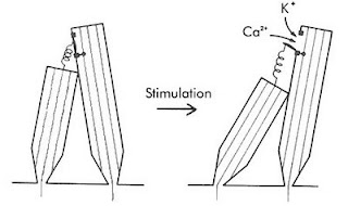
The genesis of generator potentials in the hair cells is also interesting. Imagine that a group of persons of varying height are standing on a carpet. A thread is attached from the top button (of his shirt) of the smaller person to the top button of his taller counterpart. If the carpet is now tilted by pulling it up from the short person’s end, the thread will now be stretched snapping the taller person’s button. The hair cells also have threads (Tip Links) extending from shorter to their taller cousins. A traveling wave will cause pulling of tip links, resulting in the opening of a mechanically sensitive cation channel. Since potassium is the predominant cation in the endolymph, K+ will then enter the taller hair cells. Look at the electrical gradient around the hair cell; it is -140mV with respect to the endolymph (it is about negative 60 mV wrt the perilymph). So, cations, specially K+ rushes in  creating depolarization. A cascade of events like opening of voltage-gated Ca++ ion channels at the base, consequent fusion and exocytosis of vesicles discharging neurotransmitters, probably glutamate to the afferent cochlear nerve endings surrounding the hair cells, creating an action potential in the nerve.

Frequency Discrimination
When we listen to music, our ears pick up the frequencies in a number of ways. Firstly, the place (maxima) on the BM where maximum excitation takes place is actually a function of frequency. As a matter of fact, there is a frequency map along the BM. Secondly, at frequencies below 3 kHz, the nerves fire in synchrony with the incident sound waves. This is called the ‘volley principle’. The ‘phase locking’ of the two frequencies that occurs below 3 kHz, is highly analogous to the ‘phase locked loops’ in electronic circuits (NE565). Thus ‘volley principle’ allow us to discriminate frequencies. Actually, volley effect is more important in ‘loudness’ assessment. ‘Pitch’ (the subjective/psychological dimension related to frequency) are also moderated by factors such as loudness and the duration of sound. At low frequency (below 500 Hz) pitch seems lower and at higher frequencies (above 4 kHz) pitch seems higher, as the loudness increase, when the frequency is kept constant. Again, when the duration of sound increase from 0.01 second to 0.1 second, the pitch will rise too, for a particular frequency. Sound of less than 0.01 sec duration does not evoke appreciation of any pitch by us.

Loudness Discrimination
Loudness is the perceived intensity of sound, a subjective psychological dimension. The interpreted sound sensation is proportional to the cube root of the actual sound intensity. As such, the ear works at the top of its limit, at a point analogous to Hopf bifurcation, beyond which instability in oscillations occur.
As the sounds become louder, the amplitude of BM movement is more, resulting in more excitation of hair cells. Secondly, with greater loudness, the hair cells around the ‘maxima’ fire too. This causes spatial summation. Thirdly, the outer hair cells are stimulated at loud sounds. The brain will automatically infer loudness levels when cells corresponding to the outer hair cells fire.

Locating Sounds
Then there is location of the direction of sound. We can locate whether the drums are on the left and the lead guitar is to the right. This is achieved by calculating which ear gets the sound first (time lag) and/ or which ear gets it louder (intensity). The time lag method works below 3 kHz; while intensity method works at higher frequencies.
Front/ back discrimination is done by the pinna (auricle) of our ears due to their particular shape.

Auditory nerve
It is interesting that each auditory nerve fiber has its own characteristic frequency, the frequency at which it responds most well. However, it is true only at low intensity. At higher intensities, this specificity is lost and they then respond to a wider spectrum of frequencies. The auditory nerve produces a flurry of action potentials, the frequency of which depends on the intensity of the sound stimuli, it is exposed to. This is very much similar to ‘voltage to frequency converter’ ICs (LM331 is one such VFC IC), where a change in voltage at the input of VFC will cause a change in frequency at the output.

The auditory nerve then goes to the: cochlear nucleus in the medulla to Superior olivary nucleus to Inferior colliculus (via lateral lemniscus) to Medial Geniculate Body (in the Thalamus) to end in Auditory cortex. Some fibers cross to the other side early in their course while others cross at other levels. Fibers from primary auditory area sends association fibers to different parts of the brain for language processing and other tasks.
The nerve synapses with higher order neurons in the above places, which then relay to the nerves upstream. Everywhere in its course, including the nuclei, there are clearcut ‘tonotopic maps’, representing definitive frequency layouts. There are also extensive crossing of nerve fibers to the opposite side. Before the fibers reach the auditory cortex, they connect to many reflex pathways vital to life. For example, they send branches to the reticular activating system which keeps us awake during the noisy hours.

The auditory cortex (Brodmann’s area 41) is the portion of the cerebral cortex in the superior temporal gyrus. Its anterior part is mainly concerned with low frequency and the posterior part tackles the higher frequencies. Thus area 41 also has its own tonotopic map. Secondary auditory cortex (auditory association area) is vital for the interpretation of sounds. A person, in whom Wernicke’s area (part of auditory association area) is damaged, will hear normally but will fail to understand its meaning, leading to aphasia.

The sheer complexity of the auditory circuitry is really mind-boggling: the logarithms (we hear in a log scale, not a linear one), cube functions, phase locking are only some of them. The range of sound intensity (from whisper to the roar of a jet plane) we hear is about 1 trillion fold; but surprisingly, the auditory nerve fibers have a much less dynamic range. Yet we hear the full range. It’s really amazing.


P. Martin (2001). Compressive nonlinearity in the hair bundle's active response to mechanical stimulation Proceedings of the National Academy of Sciences, 98 (25), 14386-14391 DOI: 10.1073/pnas.251530498

Last modified: Mar 10, 2014
Reference: Textbook of Medical Physiology, 17e, Guyton and Hall

Generation Of Cardiac Rhythm

The heart is vital to our bodies, since it pumps blood into various parts of our bodies, that provide us oxygen, nutrients and takes away the metabolites for disposal. For this, the heart has to contract in order to generate enough force for the ventricles (atria too) to have a standard ejection fraction. Not only does it contract, it also generates the impulses necessary for its contraction, a property called automaticity, by which it generates its own rhythm.

The cells in our bodies are bathed in a sea of fluid. This fluid, called the extracellular fluid or ECF, as it is located outside the cells. The ECF is rich in sodium ions (Na+), while their concentration inside the cells are much less. Conversely, the concentration of potassium ions (K+) is more inside than outside. It is due to this difference in concentration of ions on either side of the cell membrane, a transmembrane voltage is produced. These ions being polar in nature and water soluble, can not penetrate the lipid cell membrane. But they can gain entry, through specialized pores called ion channels.

The sodium ion channels, channels through which sodium ions pass, has 2 gates: an activation gate and an inactivation gate. What controls these gates is not known for sure, but it could either be an energy barrier controlling its entry or a flexible peptide chain-like stuff that alters the conformation of the gates to restrict the ion's access. Extracellular calcium ions also restrict sodium ions to go through and thus has a stabilizing effect. These gates are called voltage controlled gates, since the opening or closure of the gates are controlled by transmembrane voltage. These gates are inactivated at voltages above -55mV (i.e. say -40 mV) and no sodium ion can pass. Below -70 mV , the gates are open, allowing free flow of Na+ along the electrochemical gradient, from the exterior to the interior of the cell.

There are areas of heart other than the sinus node which have intrinsic automaticity i.e. they are capable of generating their own rhythms, such as the Purkinje fibers. But the SA Node (sinoatrial node) is the normal pace-maker, since it fires at the highest rate. In the nodal tissue, where the cell voltage hovers around -60 to -55 mV (millivolt), the sodium ion channels are inactivated at this voltage. Since, the resting membrane potential (RMP) of the pacemaker lies in a region where the sodium channels are inactivated, the firing of the SA Node depends on other ions, particularly calcium ions (Ca++). These nodal pacemaker cells (possibly P cells, containing little organelles) are inherently 'leaky' to calcium ions. So, Ca++ enters these cells making the cells' interiors less negative, (Ca++ is a cation bearing 2 positive charges. A cation is a positively charged ion, so called because it is attracted towards the cathode). Once the cell gains enough positive charge, to become a little more positive, about -40 mV, as shown in the figure (prepotential), there is a sudden spurt of calcium influx (impulse). T type (transient) calcium channels are responsible for the prepotential while L (long lasting) type calcium channels are responsible for the impulse. In addition to the influx of calcium ions from the ECF, calcium is also liberated locally from the sarcoplasmic reticulum of the nodal cells, known as the 'calcium spark'. So, the cell is now fully depolarized, as shown. But soon calcium channels close and influx stops. Potassium channels open. Since the concentration of K+ is more inside, K+ leaves the cell making the interior more negative. The efflux of K+ and stopping of further influx of Ca++ repolarizes the cell, making it ready for another cycle. Ca++ leaks again and the cycle repeats.

The colored animation on the top left shows the spread of cardiac impulse, from the SA Node. Click on the animation if it doesn't animate on its own.

Last modified: Mar20 2009
Reference: Basic and Clinical Pharmacology, Bertram G Katzung, 9th ed, page 220

Spiny Dendrites

The significance of dendrites, neuronal processes, so far thought of only as 'passive components' in the brain circuitry are now being discovered anew. It was known that dendrites could be depolarized to form generator potentials (normally the inside of a cell is negative with respect to the outside. This potential difference or gap in cell voltage, is decreased when a generator potential is established), but it was later found out that they could also produce action potentials (this means that the voltage change was not restricted locally, it spread to other parts of the cell). It was thought that dendrites merely added the multiple inputs algebraically, that is, it acted like an integrator in an electronic circuit. But it was discovered that they were also capable of modifying the signals in a number of ways and they were not just extensions of the soma (cell body of the neuron) so that dendrites only contributed more surface area that were available for integration or synapse formation.

It is now known that dendrites play a very vital role in memory formation and maintenance in addition to its possible role in producing consciousness. Dendrites have tiny knob-like processes on their membranes called dendritic spines. The number and the thickness of these spines vary with age and in disease. For example, in Down's syndrome (or trisomy 21) the spines are thin and small. Their shapes and sizes change in a matter of minutes to hours. They also produce proteins using mRNAs that had migrated from the soma. These mRNAs latch onto ribosomes situated on the dendritic spines and produce proteins. These proteins modify the effects of the input of glutamatergic (glutaminergic) neurons on them. This alters NMDA and AMPA receptor activities. Long term potentiation (LTP) and thus learning is affected by the rearrangement of these spines.